Word2Vec : Skip-gram with Negative Sampling
Introduction
When I wanted to build a recommendation algorithm, I came across Word2Vec and more specifically the SGNS (Skip-Gram Negative Sampling) variant. Instead of simply using a ready-made model (like gensim) that I barely understood, I thought: why not recode everything from scratch to truly grasp what’s going on under the hood.
The original Word2Vec consists of word embedding to capture semantics (checking whether words share similar meanings). This model can be extended to other domains, such as music recommendation, by treating a playlist as a sentence and a song as a word for example. Here, however, we will implement the original W2V and focus on words, not music.
The challenge was all the more interesting given that I found no from-scratch implementation of SGNS anywhere (only code using PyTorch, which abstracts away quite a lot…). I therefore relied mainly on the original SGNS paper and various incomplete implementations found online.
Model
The beginning
Here we focus on Word2Vec Skip-gram: we start from a center word and want to predict the “context”, ie the surrounding words. (W2V CBOW does the opposite: predicts the center word from the context).
Word2Vec is a small neural network, but one we won’t use for classification: we’ll train our model to predict the probability that a word is close to another, but the final result is the input weight matrix, which becomes the embedding matrix. That’s the subtle part!
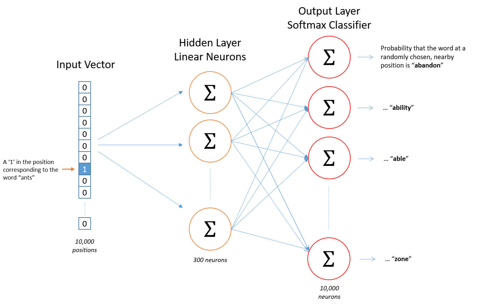
The picture shows the idea behind Skip-Gram. It’s far from the actual implementation, but it’s a useful detour to build intuition. We consider a vocabulary of 10k words and will produce embeddings of dimension 300 (reducing from 10k down to 300).
We take a word represented as a vector (we’re doing embedding), it goes through a first layer that captures important information (going for example from dim=10000 to dim=300). We’ll call the weight matrix tied to this layer $W_{in}$, the input embedding matrix. This matrix holds the information about words when they play the role of “center” (we’ll use $W_{in}$ as our embedding matrix). This is the matrix we actually care about — and we can see the embedding happening here: we’ve reduced the dimension and extracted meaningful information.
Then, we pass our vectors through the final layer, associated with weight matrix $W_{out}$, the output embedding matrix. We then apply a softmax on the final vector to get probabilities. This vector has dimension 10k — the vocabulary size — and each component corresponds to the probability that word i is close to “ants” in our example.
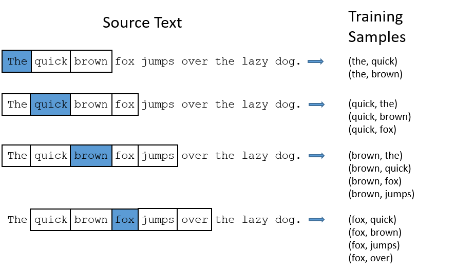
In our sentences, the window of words considered as context is a parameter: you can tell the model to look at only 2 words around the center word, or up to 10. In practice, this window is random (uniformly sampled between 1 and the value given as parameter). This means a word can have 1, 2, …, up to the maximum window size (R) of words around it. We take up to R words to the left and R words to the right, while respecting: sentence boundaries, sentence segmentation (we don’t cross a “.”, “?”, “!”).
This dynamic window matters: it reduces overfitting on immediate neighbors and introduces controlled noise that stabilizes SGNS. It’s also what Mikolov uses in the original implementation. Here’s an example of training data extraction from a sentence to make things clearer (center, context):
The loss we care about is a sum over the negative logs of these probabilities:
\[p(w_O \mid w_{I}) = \frac{\exp({v'_{w_O}}^\top v_{w_I})} {\sum_{w=1}^{W} \exp({v'_w}^\top v_{w_I})}\]I for the center word, O for the context word and W the number of words in the vocabulary.
We can see that for each term in the sum, we’ll need to sum over the entire vocabulary…
We also notice that the neural network is huge (we have 10k output neurons since the vocab size is 10k here), meaning each matrix would have 3 million components (weights)! The loss is also expensive to compute since we have to sum over the entire vocabulary multiple times at each step.
The main problem is computational cost: for each (center, context) pair, we need to sum over the entire vocabulary in the softmax and update a large number of weights. This is way too slow for large vocabularies.
That’s why we use negative sampling (SGNS for Skip-Gram Negative Sampling).
Negativ sampling
Instead of updating our entire weight matrix at each training sample as we’re currently doing (the loss depends on every word in the vocabulary), we’ll only update a small subset, but smartly.
Taking the training sample examples from above and considering “fox” as the center word, positive samples would be “brown”, “jumps” while negative samples would be “horse”, “table”.
Negative samples are words that don’t appear in the context of the center word, chosen randomly from the vocabulary, while positive samples are words we want the center word to be close to.
Our loss becomes:
\[\mathcal{L}(c,o,\{n_i\}_{i=1}^K) = - \log \sigma(\mathbf{v}_o^\top \mathbf{v}_c) -\sum_{i=1}^K \log \sigma(-\mathbf{v}_{n_i}^\top \mathbf{v}_c).\]Where $n_{i}$ are the negative sample words, $v_{c}$ is the center vector and $v_{o}$ is the positive (context) vector.
Note that $v_{c}$ lives in matrix $W_{in}$ and $v_{o}$ lives in matrix $W_{out}$.
We went from a global loss to a sample-specific loss for each training sample (1 training sample = 1 (center, context) pair) that we want to minimize. Here K is the number of negative samples we decide to use per training sample (typically K between 5 and 20, per the Word2Vec paper), it’s a hyperparameter of the model, fixed throughout training.
We’re no longer summing over the entire vocabulary, which drastically cuts down computation time, since we won’t update all weights per sample. Instead, we’ll update K+2 vectors (center, context and the negative samples).
To randomly draw these negative samples, we use a modified unigram distribution (with a 3/4 exponent) where for word $w_i$:
\[P(w_i) = \min(\frac{ f(w_i)^{3/4} }{ \sum_{j=0}^{|Vocab|} f(w_j)^{3/4} },1)\]The 0.75 exponent smooths the distribution: it slightly reduces the weight of very frequent words (the, of, …) while still keeping them more likely to be sampled than rare words.
It can be shown that SGNS is closely related to the factorization of a PMI (Pointwise Mutual Information) matrix between words and contexts, which explains why the vectors capture semantic relationships so well.
Subsampling
Another element added to the base W2V model is subsampling. In English for example, some words are far more frequent than others: the, is, and, … These highly frequent words hurt the model if left as-is. We’d end up with 12000 samples for “the” as center and only 100 for “king”, and the model would basically only ever see “the” and “is”.
That’s why we use subsampling: we’ll remove a large portion of pairs to balance the dataset. The more frequent a word, the more (frequent word, context) pairs we discard. This is done through the formula:
\[P_{\text{keep}}(w) = \left( \sqrt{\frac{f(w)}{t}} + 1 \right) \cdot \frac{t}{f(w)}\]where w is a word, f(w) its frequency in the corpus and t is a model parameter (typically t=1e-5). The smaller t, the fewer words we keep — and rare words are almost always kept.
Processing
Now let’s get a bit more hands-on and start coding.
We’ll begin with data processing. In my case, the dataset is wikitext2, which is sufficient. It’s a small dataset compared to what’s available, but it lets models run in under 5 minutes on modest machines and the model still manages to extract good word relationships (Word2Vec scales extremely well). Our training data consists of (center, context) pairs extracted from sentences delimited by ., ? and !.
The code is freely available on my GitHub. I strongly recommend having it open alongside this post to follow along more easily.
text = corpus.lower()
text = re.sub(r"[^a-z0-9.,!?;:'\-()\s]", " ", text)
tokens = re.findall(r"[a-z0-9]+(?:'[a-z0-9]+)?|[.,!?;:()\-]", text)
Next, we’ll build our vocabulary and map words to IDs, since we’re working with numbers in our vectors. This is what the tokenisation function does, it also returns the word count (count) in the corpus and their relative frequencies (f_relg).
count will be used to build the sampling distribution for drawing negative samples (build_noise), and the relative frequencies (f_relg) are used for subsampling (filtre_s).
We then use this data to create our training samples (pairs) through the pair function (which uses a dynamic context window) and pairs.
Word2Vec SGNS Model from scratch
Model
Let’s start with a bit of math: What we care about is the gradient of the loss, since it tells us which direction to go to minimize it. To do this, we’ll compute the partial derivatives with respect to each component of the loss:
\[\frac{\partial \mathcal{L}}{\partial \mathbf{v}_c} = (\sigma(\mathbf{v}_o^\top \mathbf{v}_c)-1)\mathbf{v}_o + \sum_{i=1}^K \sigma(\mathbf{v}_{n_i}^\top \mathbf{v}_c)\mathbf{v}_{n_i}.\] \[\frac{\partial \mathcal{L}}{\partial \mathbf{v}_o} = (\sigma(\mathbf{v}_o^\top \mathbf{v}_c)-1)\mathbf{v}_c .\] \[\frac{\partial \mathcal{L}}{\partial \mathbf{v}_{n_i}} = \sigma(\mathbf{v}_{n_i}^\top \mathbf{v}_c)\mathbf{v}_c, \qquad i=1,\dots,K.\]We can now update matrices $W_{in}$ and $W_{out}$ as we go through the samples. This is what we see in the train method of the Word2Vec class:
neg_ids = self.sample_negatives(self.K, rng)
neg_vecs = self.W_out[neg_ids]
pos = np.dot(v_c, v_o)
pos = np.clip(pos, -10, 10) #we clip to keep convergence, 10 -10 is suffisant for the sigmoid

neg = neg_vecs.dot(v_c)
neg = np.clip(neg, -10, 10) #we clip to keep convergence, 10 -10 is suffisant for the sigmoidut

sig_pos = sigmoid(pos)
sig_neg = sigmoid(neg)

grad_c = (sig_pos - 1) * v_o + np.sum(sig_neg[:, None] * neg_vecs, axis=0)
grad_o = (sig_pos - 1) * v_c
grad_negs = sig_neg[:, None] * v_c[None, :]

self.W_in[center_id]   -= lr_t * grad_c
self.W_out[context_id] -= lr_t * grad_o
np.add.at(self.W_out, neg_ids, -lr_t * grad_negs)
We follow the gradient direction (weighted by the learning rate) and update both matrices. The np.add.at handles duplicate indices: Frequent words are more likely to be drawn as negative samples, so it’s not unusual to see the same word appear twice. To avoid underupdating these words, we add the gradients instead of overwriting them, so they accumulate rather than cancel each other out.
Model Stabilization
We use a decaying learning rate to prevent the norms from diverging (we didn’t add any vector regularization here).
Also worth noting: we shuffle the pairs (all our training data) so the model treats each pair fairly (otherwise a pair like (king, charles) might end up at the very end of training where the learning rate is at its minimum, barely getting any update).
Speed on Negative Sample Selection
Mikolov’s idea was to build a distribution table instead of using something like np.random.choice, which would be O(|Vocabulary|). We create a huge table where each position corresponds to a word. How many times a word appears in the table is proportional to its probability of being drawn as a negative sample. This brings us down to O(1).
Comparison and Metrics
We can compute an average loss on a subset of words and check at each epoch whether it decreases, but I relied on cosine similarities and the 20 nearest neighbors of words like “king” or “football” to assess whether my model was actually learning meaningful things. Here’s the cosine similarity formula:
\[\cos(u, v) = \frac{u \cdot v}{\|u\|_2 \, \|v\|_2}\]Results
Here are the parameters I used for the results I’m about to show you. The model is saved on my GitHub and the code is fully functional so you can train your own (I didn’t do any hyperparameter optimization). I also normalize $W_{in}$ before finding the k nearest neighbors.
- window_size_max = 3
- embed_dim = 300
- negatives = 5
- lr_initial = 0.025
- epochs = 5
- t = 1e-3
Top 10 neighbors for ‘king’:
| Word | Score |
|---|---|
| henry | 0.7735 |
| william | 0.7537 |
| george | 0.7510 |
| james | 0.7244 |
| son | 0.7180 |
| john | 0.7088 |
| edward | 0.7079 |
| richard | 0.7008 |
| charles | 0.6987 |
| michael | 0.6868 |
Analogy [king - man + woman] vs queen (cosine): 0.6920
king $= [ 0.2738726 , -0.1502892 , -0.11983082 , -0.0713472 , -0.07030658] $
queen $= [ 0.15040387 , -0.00734318 , -0.02329289 , -0.09677064 , -0.10576637]$
Top 10 neighbors for ‘football’:
| Word | Score |
|---|---|
| championship | 0.8472 |
| cup | 0.8328 |
| rugby | 0.8279 |
| tag | 0.8254 |
| baseball | 0.8085 |
| conference | 0.8075 |
| premier | 0.8009 |
| league | 0.8007 |
| fa | 0.7895 |
| liverpool | 0.7843 |
| finals | 0.7826 |
We can clearly see that our model has learned semantic relationships, and the results are genuinely solid compared to optimized models like Gensim. The cosine similarity for the King vs Queen analogy is 0.61 for Gensim, our model has apparently captured the relationship between king and queen better. Gensim does return slightly more relevant results overall though:
Top 10 neighbors for ‘football’ from Gensim:
| Word | Score |
|---|---|
| basketball | 0.8902 |
| athletic | 0.8893 |
| rugby | 0.8882 |
| baseball | 0.8821 |
| hockey | 0.8784 |
| yeovil | 0.8662 |
| wheelchair | 0.8638 |
| conference | 0.8585 |
| coaches | 0.8581 |
| aston | 0.8513 |
The similarity scores are higher for some sports, but our model clearly holds its own and successfully captures semantic structure!!!!!