Mind the dual gap, LASSO
Introduction
The classical LASSO solver based on coordinate descent quickly becomes expensive when the number of variables is much larger than the number of observations ($p≫n$).
Modern implementations speed up this solver using screening rules, which safely eliminate variables whose optimal coefficient is zero.
In this post, I implement and explain the paper Mind the Duality Gap: Safer Rules for the Lasso, which leverages the duality gap to build convergent safe regions and significantly reduce the cost of the solver.
I primarily relied on Convex Optimization by Boyd and Vandenberghe to acquire the background needed to implement and understand this paper.
A bit of theory
Before understanding what the paper does and why it works, let’s first change perspective on the LASSO.
Recall that the primal LASSO problem is:
\(\hat{\beta}(\lambda) = \arg\min_{\beta} \left( \frac{\| y - X\beta \|_2^2}{2} + \lambda\| \beta \|_1 \right)\) where $X \in \mathbb{R}^{n\times p}$ and $\beta \in \mathbb{R}^{p}$.
By splitting between residuals and features (we set $\rho = y - X \beta$ for the primal problem) and using the Lagrangian:
\(L(\rho,\theta, \beta)=\frac{\|\rho \|_2^2}{2} +\theta^{T}((y-X \beta)-\rho) + \lambda \| \beta \|_1\) where $\theta$ is the dual variable.
After minimizing over $\rho$ and $\beta$, we obtain the dual problem:
\(\hat{\theta}(\lambda) = \arg\max_{\theta' \in \Delta_X} \frac{1}{2}\|y\|_2^2 - \frac{\lambda^2}{2} \left\| \theta' - \frac{y}{\lambda} \right\|_2^2 =\arg\max_{\theta' \in \Delta_X} g(\theta')\) where $\Delta_X = {\theta’ \in \mathbb{R}^n : |x_j^\top \theta’| \le 1,\ \forall j \in {1,\ldots,p}}$ is the dual feasible set, with $\theta’=\frac{\theta}{\lambda}$ (the constraint arises from minimizing over $\beta$).
We observe that the dual problem reduces to: \(\hat{\theta}(\lambda) = \arg\min_{\theta' \in \Delta_X} \left\| \theta' - \frac{y}{\lambda} \right\|_2\)
so $\hat{\theta}(\lambda)$ is the projection of $\frac{y}{\lambda}$ onto $\Delta_X$ under the Euclidean norm. Since $\Delta_X$ is convex and closed, this projection is unique by theorem.
The solution to the primal problem is not necessarily unique (depending on the rank of X).
Note also that at the optimum, $\lambda\hat{\theta}(\lambda)+X\hat{\beta}(\lambda)=y$, accounting for the normalization by $\lambda$.
In what follows we write $\theta$ instead of $\theta’$, even though it refers to the normalized version.
Applying the KKT conditions to $L(\rho,\theta, \beta)$, we obtain conditions on the $\beta_j$ (similar calculations were carried out in my previous post):
The dual problem yields a unique solution and simple geometric conditions — the only catch is that we do not know the dual solution!
Screening rules
Our goal here is to safely eliminate useless variables. A variable $\beta_j$ is useless when: \(|x_j^{T} \hat{\theta}(\lambda) |<1\)
The key idea is that since we do not know the dual solution, we look at sets $C$ that are slightly larger but contain it (these sets are called safe regions), and require a stronger property.
If that property holds, we can discard the variable $\beta_j$ without knowing the dual solution.
This property is our safe rule: \(\mu_C(x_j):= \sup_{\theta \in C} |x_j^{T}\theta| <1\)
Since the dual solution lies in $C$, we know for certain that $\beta_j=0$.
We have not yet defined $C$, but we see that if $\mu_C(x_j)$ can be computed explicitly and efficiently, the computation will be lightweight.
To achieve this, $C$ must be chosen carefully: simple enough (to keep the cost of evaluating the safe rule low) and as small as possible (to eliminate as many useless variables as possible).
The paper uses a particular ball, though domes and other geometric shapes have also been explored in the literature.
If we use a single fixed set $C$ just before the solver, we have a static rule.
The paper proposes a dynamic rule that acts at each step of the (iterative, coordinate descent) solver, providing a sequence of sets that converges (in the sense that the diameter tends to zero) towards ${ \hat{\theta}(\lambda) }$.
Mind the duality gap
Getting started
For a ball $B(c,r)$, we have $\mu_C(x_j)=|x_j^{T}c|+r|x_j|$.
The paper uses the duality gap to find a suitable sequence of balls.
Indeed, for any primal/dual feasible pair, weak duality holds. Since Slater’s conditions are also satisfied here, we further have strong duality: \(\frac{1}{2}\|y\|^2 - \frac{\lambda^2}{2} \left\|\theta - \frac{y}{\lambda}\right\|^2 \le \frac{1}{2}\|X\beta - y\|^2 + \lambda \|\beta\|_1\) for $\theta \in \Delta_X$!
We therefore extract a lower bound on $|\theta - \frac{y}{\lambda}|$ for any $\theta \in \Delta_X$, and in particular for $\hat{\theta}(\lambda)$: \(\left\lVert \theta - \frac{y}{\lambda} \right\rVert \ge \frac{\sqrt{\left(\lVert y \rVert^2 - \lVert X\beta - y \rVert^2 - 2\lambda \lVert \beta \rVert_1\right)_+}}{\lambda} =\hat{R}_{\lambda}(\beta)\)
Now fix a point $\theta \in \Delta_X$. Then $\tilde{R}_{\lambda}(\theta)= |\theta - \frac{y}{\lambda}| \geq |\hat{\theta}(\lambda) - \frac{y}{\lambda}|$ by definition of the projection.
Thus the dual solution lies in the annulus: \(\hat{\theta}(\lambda) \in A\!\left(\frac{y}{\lambda},\tilde{R}_{\lambda}(\theta),\hat{R}_{\lambda}(\beta)\right)\)
Geometric intuition
The duality gap tells us that the dual solution $\hat{\theta}(\lambda)$ lies in an annulus centered at $\frac{y}{\lambda}$, but this information is too coarse: an annulus is not a simple or convenient shape for screening.
We will exploit the convex structure of the problem to derive a suitable ball.
Recall that $\hat{\theta}(\lambda)$ is the projection of $\frac{y}{\lambda}$ onto $\Delta_X$, which is convex and closed, so the segment $[\theta,\hat{\theta}(\lambda)]$ stays inside the set. Since $\hat{\theta}(\lambda)$ is the point of $\Delta_X$ closest to $\frac{y}{\lambda}$, this segment cannot enter the inner ball of the annulus (whose radius is given by the duality gap).
$\hat{\theta}(\lambda)$ is therefore geometrically constrained, and the farthest point from $\theta$ that is compatible with these constraints is obtained when the segment from $\theta$ is tangent to the inner ball. This point is denoted $\theta_{int}$ in the paper and gives our safety radius.
We thus obtain a ball centered at $\theta$ that contains the dual solution.
In conclusion, the safe region is: \(C'=B\!\left(\theta,\left(\tilde{R}_{\lambda}(\theta)^2 - \hat{R}_{\lambda}(\beta)^2\right)^{1/2}\right)\) where the radius equals $|\theta_{int}-\theta|$ (see Figure 1).
What is $\theta$?
A brief note on the $\theta$ we fixed earlier.
Above, we assumed we have some $\theta \in \Delta_X$, but we still need to actually choose one.
From the KKT conditions on the dual problem, we know that $\hat{\theta}(\lambda)$ is proportional to the residual. At step $k$ we therefore build $\theta_k$ from the residual $\rho_k = y - X\beta_k$ and a constant $\alpha_k$ chosen so that $\theta_k = \alpha_k \rho_k \in \Delta_X$.
We pick $\alpha_k$ as the best scaling of $\rho_k$ that remains dually feasible — in other words, the projection of the unconstrained optimal coefficient onto the feasibility interval imposed by $\Delta_X$.
Building the safe region
Let $r’(\theta,\beta)$ denote the radius of the chosen ball.
We have $r’(\theta,\beta)^2 \leq r(\theta,\beta)^2:= \frac{2}{\lambda^2}G(\theta,\beta)$, where $G(\theta,\beta)$ is the duality gap, and $r(\hat{\theta}(\lambda),\hat{\beta}(\lambda))=0$ by strong duality.
We use the duality gap as the radius rather than the geometrically derived one, because the duality gap is a standard stopping criterion in solvers and is therefore already computed. Indeed, if $G(\theta,\beta) \leq \epsilon$, then by strong duality $P_{\lambda}(\beta)-P_{\lambda}(\hat{\beta}(\lambda)) \leq \epsilon$.
This makes it numerically convenient.
We therefore set $C=B(\theta,r(\theta,\beta))$.
Since our radius is built from $G(\theta,\beta)$, if the solver converges to $(\hat{\theta}(\lambda),\hat{\beta}(\lambda))$, the radius tends to zero.
Thus $C_{k}=B(\theta_k,r(\theta_k,\beta_k))$ is a safe region that converges to ${\hat{\theta}(\lambda)}$ as $\lim(\theta_k,\beta_k)=(\hat{\theta}(\lambda),\hat{\beta}(\lambda))$.
Implementation
The paper provides pseudocode that nonetheless requires careful adaptation (vectorization and removal of redundant computations), since on large datasets like Leukemia, inefficiencies are very costly.
You can find the full code in my GitHub repo!
Recall that the algorithm runs inside the solver, but the solver itself does not change. The coordinate descent algorithm is unchanged: we simply add screening that removes passive variables so that the solver only updates the active ones.
Here is the pseudocode from the paper: 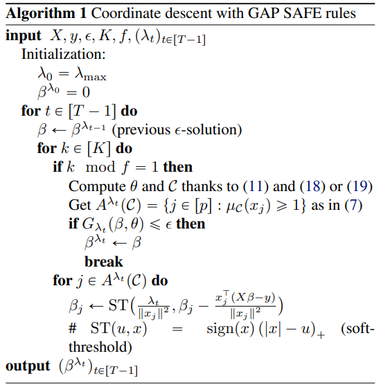
I did not mention warm-starting earlier: it consists of initializing $\beta_{k+1}$ from $\beta_k$ rather than from zero (this is valid in practice because for two close values of $\lambda$, the successive LASSO solutions are generally close. This makes warm-starting very effective along the regularization path).
I omit the __init__ function here, which is identical to the one in my previous post except that I moved the target y and its standardized version yc into it.
The f parameter in the pseudocode controls how often screening is performed. Screening does carry a cost, so running it at every epoch is unnecessary.
Following the pseudocode, we start by computing the active/passive set and $\theta$:
    def gap(self,beta,theta,a,rho):
        Gap = max((
            0.5 * np.sum((rho)**2)
            + a * np.sum(np.abs(beta))
            - 0.5 * np.sum(self.yc**2)
            + 0.5 * (a**2) * np.sum((theta - self.yc / a)**2)), 0.0)
        return Gap

    def safe_active_set(self,theta,beta,a,rho):
        gap = self.gap(beta,theta,a,rho)
        r = np.sqrt(2 * gap)/a
        scores = np.abs(self.Xc.T @ theta) +
                r * np.sqrt(self.Xn2)

        active = np.where(scores >= 1)[0]
        z_passiv = np.where(scores < 1)[0]
        return active,z_passiv

    def compute_theta(self,rho,active,a):

        if len(active)==0:
            return np.zeros_like(rho)

        m = np.max( np.abs( self.Xc[:, active ].T @ rho ))

        if m == 0:
            return np.zeros_like(rho)

        alpha0 = np.dot(self.yc, rho) / ( a * np.dot(rho, rho))
        alpha = min( max(-1/m, alpha0), 1/m )
        return alpha * rho
gap computes the duality gap — note that the residual $\rho$ is passed as an argument!
safe_active_set computes our safe region $C$ using the two functions above.
        scores = np.abs(self.Xc.T @ theta) +
                r * np.sqrt(self.Xn2)
        active = np.where(scores >= 1)[0]
        z_passiv = np.where(scores < 1)[0]
Here I vectorized the safe rule computation with NumPy, which makes a real difference on large datasets like Leukemia where $p=7000$.
We then retrieve active and z_passiv, which let us screen out passive variables and run coordinate descent only on the active set.
We then compute $\theta$ by computing $\alpha$ (with $\rho$ as an argument).
We update the residual in-place inside the CD loop, which is why it is passed as an argument to each function above. Indeed, recomputing $\rho$ from scratch is expensive when $p$ is large (even with screening), as it requires $O(n \cdot p)$ operations, whereas the residual can be updated incrementally in $O(n)$.
    def safe_gap_rule(self,tol,iter,bi,f,a):
        active = np.arange(self.p)
        beta = bi.copy()
        rho = self.yc - self.Xc @ beta
        theta = self.compute_theta(rho,active,a)
        for i in range(iter):

            if i % f == 0:

                active ,passiv = self.safe_active_set(theta,beta,a,rho)

                if len(passiv) > 0:
                    rho = rho + self.Xc[:, passiv] @ beta[passiv]
                    beta[passiv] = 0.0
                theta = self.compute_theta(rho,active,a)
                if len(active) == 0:
                    break
            if self.gap(beta,theta,a,rho)<tol:
                break
            for j in active:
                x_j = self.Xc[:, j]
                r_j = rho + x_j * beta[j]
                beta_new_j = self.s_threshold(np.dot(x_j, r_j), a) / self.Xn2[j]
                delta = beta_new_j - beta[j]
                rho = rho - x_j * delta
                beta[j] = beta_new_j
        return beta
This is the main function safe_gap_rule, which handles both screening and CD.
We start by initializing the parameters ($\rho$, $\theta$, and active, the index set of active variables).
As noted above, screening is not performed at every epoch, only when i % f == 0.
                if len(passiv) > 0:
                    rho = rho + self.Xc[:, passiv] @ beta[passiv]
                    beta[passiv] = 0
                theta = self.compute_theta(rho,active,a)
                if len(active) == 0:
                    break
We update the residual incrementally throughout the algorithm rather than recomputing it from scratch, avoiding the $O(n \cdot p)$ cost.
rho = rho + self.Xc[:, passiv] @ beta[passiv]This removes the contribution of the zeroed-out coefficients from the residual.
This step only applies when there are passive variables (len(passiv) > 0).
rho = rho - x_j * (beta_new_j - beta[j])When updating the active variables, we subtract the change in coordinate $\beta_j$.
This ensures we never recompute $y - X\beta$ in full.
Note that if len(active) == 0, we stop immediately, since we know $\beta = 0$.
The rest closely mirrors the standard CD implemented in my previous post.
Here, the duality gap serves as the stopping criterion. This is more principled than the naive criterion based on coefficient variation, and it is already computed inside the algorithm to build the safe region.
Results
On the Leukemia dataset, the implementation with dynamic screening significantly reduces computation time compared to a naive coordinate descent in pure Python/NumPy (from over 10 minutes down to 80 seconds).
It remains considerably slower than sklearn, which benefits from a highly optimized low-level implementation.
The goal here is therefore not to compete with sklearn on raw speed, but to correctly reproduce the paper’s idea and demonstrate its concrete impact on the solver.
Below is the LASSO path produced by our code, which matches the one obtained with sklearn: 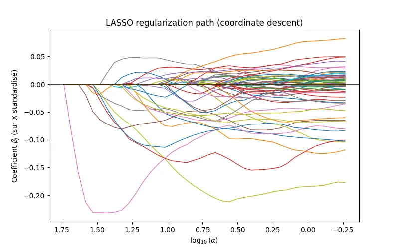
Resources
- Convex Optimization, Boyd and Vandenberghe
- A. Ndiaye, O. Fercoq, A. Gramfort, J. Salmon.
Mind the Duality Gap: Safer Rules for the Lasso.
ICML 2017.
https://arxiv.org/abs/1505.03410