Regression LASSO
Introduction
After studying Ridge in depth, let’s now look at its alter ego: Lasso, or Least Absolute Shrinkage and Selection Operator. We saw that Ridge pulled coefficients toward 0 but never actually zeroed them out. Lasso, on the other hand, can eliminate variables entirely, in other words, it selects variables and keeps only the significant ones. Lasso is a regularization model and some coefficients will therefore be exactly 0.
LASSO
Model
Instead of L2 regularization as in Ridge, LASSO uses L1 regularization:
\(\hat{\beta}_{\text{lasso}} = \arg\min_{\beta} \left( \frac{\| y - X\beta \|_2^2}{2} + \lambda\| \beta \|_1 \right)\) where $X \in \mathbb{R}^{n\times p}$ and $\beta \in \mathbb{R}^{p}$
This time we can’t solve this problem with an explicit closed form like Ridge or OLS, at least not directly… We could add a $\frac{1}{n}$ factor (also omitted in the Ridge problem) which makes $\lambda$ independent of the dataset size, enabling comparisons across datasets. Here we leave it out to keep the expression simple and since we’re not comparing across datasets. This means $\lambda$ scales with dataset size.
Solution Approach
Several algorithms exist with varying performance, but we choose standard coordinate descent here. Scikit-learn uses safe screening gap coordinate descent, which draws on convexity, duality and other concepts that go beyond the scope of this post (consider reading the next post about safe screening gap).
So we’ll just use plain coordinate descent. The idea is that even though LASSO has no explicit global solution, it does have one in 1 dimension. We therefore optimize not globally, but variable by variable, iterating over all variables.
Let’s derive the explicit solution for a single coordinate $\beta_{j}$ where $j \in {1,\dots,p}$. The problem can be rewritten as:
\[\hat{\beta}_{j} = \arg\min_{\beta_{j}} \left( \frac{\| y - X_{-j}\beta_{-j} - \beta_{j}x_{j} \|_2^2}{2} + \lambda |\beta_{j}| \right) =\arg\min_{\beta_{j}}(\rho(\beta_j))\]With $X=(x_1,\dots,x_p)$, $\quad X_{-j}=(x_1,\dots,x_{j-1},0,x_{j+1},\dots,x_p)$ and $\beta_{-j}$ the vector $\beta$ without $\beta_j$. Note that $X_{-j}\beta_{-j}$ is a sum of vectors, and letting $r_{j}=y - X_{-j}\beta_{-j}$, $\quad \mathbf{r_j}$ is independent of $\mathbf{\beta_j}$.
To be clear on notation: $x_j= (X_{1,j},\dots,X_{n,j})$
Since the absolute value is not differentiable at 0, we use the notion of subgradient to compute the gradient of $\rho$, then apply Fermat’s condition to find the explicit formula for $\beta_j$.
\[\partial |x| = \begin{cases} \{-1\} & \text{if } x < 0 \\ \{1\} & \text{if } x > 0 \\ [-1,1] & \text{if } x = 0 \end{cases}\]It’s this interval $[-1,1]$ that allows coefficients to be exactly 0 for certain values of $\lambda$, which we’ll understand in a moment. Differentiating $\rho$, we get:
\[\partial \rho(\beta_j) = \begin{cases} \{-\lambda+\beta_j \|x_j\|_2^2- x_{j} ^ \top r_{j}\} & \text{if } \beta_j < 0 \\ \{\lambda +\beta_j \|x_j\|_2^2- x_{j}^\top r_{j}\} & \text{if } \beta_j > 0 \\ [-\lambda-x_{j}^\top r_{j},\lambda-x_{j}^\top r_{j}] & \text{if } \beta_j = 0 \end{cases}\]Applying Fermat’s condition, we conclude that:
\[\beta_j \|x_j\|_2^2 = \begin{cases} \lambda+x_{j}^\top r_{j} & \text{if } x_{j}^\top r_{j} < -\lambda \\ -\lambda+x_{j}^\top r_{j} & \text{if } x_{j}^\top r_{j} >\lambda \\ 0 & \text{if } \lambda \ge |x_{j}^\top r_{j}| \end{cases}\]The third case is what gives us the condition for a coefficient to be purely zero, depending on the value of $\lambda$ relative to the data. Dividing by $|x_j|_2^2$ and compacting the expression:
\[\beta_j=\operatorname{sign}(x_{j}^\top r_{j})\frac{\max(0,|x_{j}^\top r_{j}|-\lambda)}{\|x_j\|_2^2}\]Don’t forget that the residual $r_j$ depends on the coefficients $\beta_{-j}$. Therefore, the update of $\beta_j$ is performed while treating all other coefficients as fixed. The coordinate descent algorithm consists of successive passes over the coordinates, updating each coefficient one at a time.
We use a simple convergence criterion based on a maximum number of iterations, corresponding to a fixed number of passes over all $p$ coefficients (say $m$ passes). Although convergence of coordinate descent is guaranteed for the LASSO problem, finer criteria such as KKT conditions or safe screening gap methods are not used here.
Numerical Solution
Let’s get into the code:
def __init__(self,X):
        self.X       =  X
        self.mu_X    =  self.X.mean(axis=0)
        self.sigma_X =  self.X.std(axis=0, ddof=0)
        self.sigma_X[self.sigma_X == 0] = 1.0
        self.Xc      =  (self.X - self.mu_X) / self.sigma_X
        self.n,self.p=np.shape(self.Xc)
        self.Xn2 = (self.Xc ** 2).sum(axis=0)
As usual we center and normalize X. We also create Xn2 which corresponds to the vector $x’=(|x_1|_2^2,\dots,|x_p|_2^2)$.
def s_threshold(self,z, a):
        return np.sign(z) * max(abs(z) - a, 0.0)

def cd_lasso(self,iter,a,y,b_i,tol):
    y = np.asarray(y).reshape(-1)
    yc= y - y.mean()
    beta = b_i
    for i in range(iter):
        beta_old= beta.copy()
        for j in range(self.p):

            x_j=self.Xc[:,j]

            r_j=yc-self.Xc@beta+x_j*beta[j]

            xr=np.dot(x_j,r_j)

            beta[j]=self.s_threshold(xr,a)/self.Xn2[j]
        if np.max(np.abs(beta - beta_old)) < tol:
          break
  return beta
We’ve omitted the intercept here since LASSO doesn’t act on it. The s_threshold function returns the optimal value of $\beta_j$ as derived earlier (up to a multiplicative factor).
cd_lasso implements the coordinate descent algorithm, we can clearly see how the $\beta_j$ are cyclically updated based on the previous iteration. We use an infinity norm criterion on $\beta$ to avoid unnecessary iterations. Moreover, since the LASSO solution path is continuous, instead of restarting each time from the same initialization (e.g. $\beta=0$), we use the $\beta$ from the previous $a$ as the starting point. More precisely, for $a_k$ and $a_{k+1}$ close to each other, $\beta(a_k) \approx \beta(a_{k+1})$.
We finish with lasso_path, which lets us confirm our theoretical results.
First, we need to choose a grid of values for $\lambda$ (in the code we use a since lambda is a reserved keyword in Python). We know that for a sufficiently large $\lambda$, the LASSO solution is zero. More precisely, letting $y_c = y - \bar y$, we define:
Then for all $\lambda \ge \lambda_{\max}$, we get $\beta = 0$. This value corresponds to a_max in the code.
def lasso_path(self,y,iter,tol):
        y = np.asarray(y).reshape(-1)
        yc= y - y.mean()
        a_max = np.max(np.abs(self.Xc.T @ yc))
        a_all = a_max * np.logspace(0, np.log10(1e-3), 200)
        beta=np.zeros(self.p)
        path=[]
        for a in a_all:
            beta = self.cd_lasso(iter,a,y,beta,tol)
            path.append(beta.copy())
        return a_all, np.array(path).T
Finally, we retrieve the path of each coefficient as a function of log(a/$\lambda$) through cd_lasso. We transposed path to make it easier to work with. Here are the results on the california_housing dataset from sklearn:
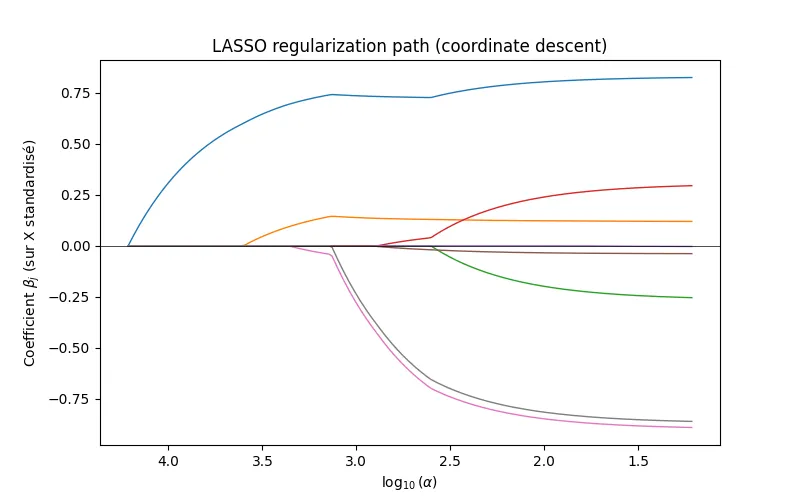
The x-axis is decreasing and logarithmic! Each curve corresponds to a coefficient, and we can clearly see that the curves don’t hit zero at the same time. Coefficients are indeed exactly 0, and the LASSO objective is achieved.
The regularization paths match those from sklearn, which validates our implementation. Our algorithm does converge more slowly due to the naive coordinate descent implementation. Since the problem is convex, the differences observed are purely numerical. It’s worth noting that coordinate descent is a numerical approximation of the optimal solution (an algorithm like LARS can give the “exact” solution), depending on our tol criterion and the conditioning of X.
Here we didn’t focus on interpreting the results or making predictions. In practice, we want to choose $\lambda$ to maximize predictive performance, cross-validation is the standard approach, picking the $\lambda$ that minimizes the loss.