DDPM

Preamble

You can find the code linked to this post on my github repo.

All of this is written by human, but AI helps me correcting mistakes and improving my markdown coloring skills.
Let’s augment the level of difficulty of this blog with some generativ modeling that will be a key part of my future work. More precisely, we’ll focus on diffusion algorithms by using first probabilistic view (DDPM: Denoising Diffusion Probabilistic Models), before attacking Consistent models and rectified Flows.
This post will be updated.

I’m not writing another post explaining the core concept and getting the equations, since a lot of amazing posts have been already made: lilan-weng, Sanderson or Yann Song.
I’ll rather tell you about what I didn’t find in these articles, my practice experience with these and what seems important to me.

Introduction

Diffusion models are generativ models that became really important after the apparition of DDPMs in 2020, especially because they progressively outperformed GANs on a lot of generativ tasks.

DDPM : The main idea

Let’s start by a small introduction on the basic model, DDPM.

Generativ models are models that want to learn a probability distribution $p_{\text{data}}$, for example an image distribution.

THe idea behind DDPM is to not learn this distribution directly. Instead, we first define a progressive noising process: we start from a real image $x_0 \sim p_{\text{data}}$, then we progressively add Gaussian noise until we get a variable $x_T$ close to pure noise $\mathcal{N}(0,I)$.

The model then learns the reverse process: starting from pure noise and progressively removing it to get back to a realistic image. In other words, instead of directly learning a very complex image distribution, we learn a sequence of small denoising steps.

This is the idea that makes the problem simpler: each step $x_t \rightarrow x_{t-1}$ is local, much easier to learn than the full transformation $\mathcal{N}(0,I) \rightarrow p_{\text{data}}$.

Le processus forward est défini par :

\[\color{orange}{ q(x_t \mid x_{t-1}) = \mathcal{N} \left( x_t ; \sqrt{1-\beta_t}x_{t-1}, \beta_t I \right).}\]

We define:

\[\alpha_t = 1-\beta_t, \qquad \bar{\alpha}_t = \prod_{s=1}^t \alpha_s.\]

A very useful property of Gaussians (called “the nice property” by L.Weng) is that we can write $x_t$ directly as a function of $x_0$:

\[x_t = \sqrt{\bar{\alpha}_t}x_0 + \sqrt{1-\bar{\alpha}_t}\varepsilon, \qquad \varepsilon \sim \mathcal{N}(0,I).\]

The network is then trained to predict the added noise:

\[\color{red}{\boldsymbol{ \mathcal{L}_{\text{simple}} = \mathbb{E}_{t,x_0,\varepsilon} \left[ \left\| \varepsilon - \varepsilon_\theta(x_t,t) \right\|^2 \right]. }}\]

A very important point is that the solution for $\color{red}{\varepsilon_\theta(x_t,t)}$ that the model should output corresponds to $\color{red}{\mathbb{E} \left[ \varepsilon \mid x_t, t \right]}$.

At generation time, we start from $x_T \sim \mathcal{N}(0,I)$, then we progressively apply the learned model to get $x_0$.

The Setup

MNIST is the classic dataset I thought was useless, because too simple, but if you use it right its simplicity is very valuable. Using MNIST and training a model on few data allows for quick experiments (a few minutes max to train) when you only have access to Colab’s GPU, and therefore quickly understand and tweak the models. It’s also interesting to design models powerful enough to work, but not powerful enough to see the model’s limits and failures.

What I learned coding DDPM

Coding the diffusion model isn’t difficult, but understanding the choices that were made, their importance and seeing them in action is more complex.

The U-net architecture is powerful

Deep Learning is used in our case to predict the noise added at time $t$, i.e. $\varepsilon_\theta(x_t, t)$, and I started simply by trying to use a MLP (neuronet in my code). I tried to optimize my MLP for 2 hours to hopefully bring the loss down, but unfortunately even on a dataset like MNIST a basic MLP has no chance on this problem:
It has to learn from scratch the structure of images (nearby pixels are likely correlated) which is what convolutions do (spatial inductive bias) and has to learn to generate images at different noise levels where it needs to give fine details at small $t$ and the global structure at large $t$…
The MLP therefore has too many things to learn on its own and without a big model, lot’s of training and data, it’s impossible to get good results.

I then moved on to building a U-net, which was much more challenging to code, but also very instructive.
The U-net was 6 light years ahead of the MLP and requires fewer parameters for what it offers.
My U-net includes some recent improvements such as $1/\sqrt{2}$ rescaling and adaGN, which give better results.
The reason lies in the U-net architecture. It learns fine details through skip connections and the global structure by doing downsampling/bottleneck, unlike a MLP.
Moreover, a U-net understands the spatial nature of images because it’s built with convolutions: spatial inductive bias (I didn’t add transformers in this first U-net) and is therefore very efficient on images and the diffusion problem while requiring little compute (compared to an equivalent MLP).

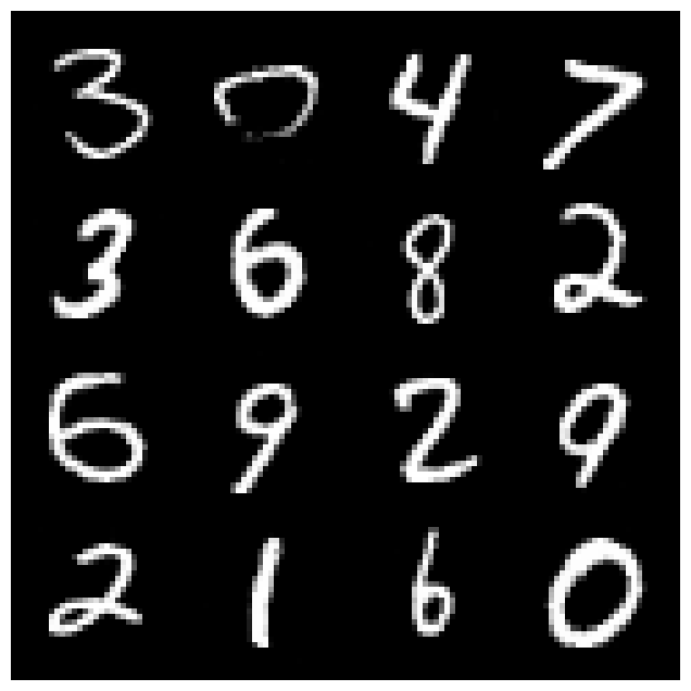
Here are some examples generated by our DDPM with random noise:

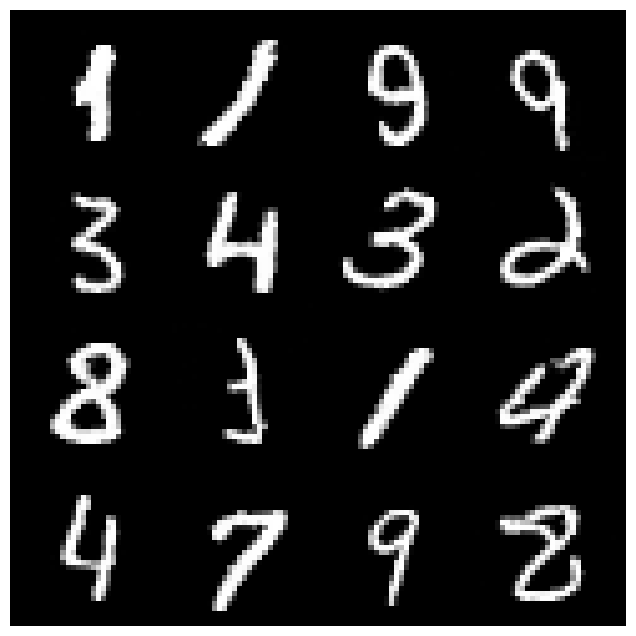1k5 images, 32-Unet, 500 epoch

Given that we train our model on only 1,500 images with a low-capacity model, I’m fairly satisfied with the result.

Time is interesting

Time seems trivial and you don’t really think about it at first (other than “the model can use time to know how much noise to add”), but 2 questions came to me.
“What happens if I remove time from my U-net?”
Time always appears in sampling with the beta-schedule, but I can remove it from my U-net’s context.
Note that time is encoded with a sinusoidal embedding, we need to feed tensors to the model.
If we remove time as the model’s context, the model takes an input and tries to denoise it without knowing a priori how noisy it is:
We can assume that a model with enough data and capacity (which isn’t really the point of this project) could capture the distribution with respect to time.
Update: some research has been made recently about this and says that it works too

DDPM is still not easy to train on a small dataset when you want to see the model’s limits with little compute, but that’s where you learn the most, I guess.

You have to keep in mind that biases accumulate during sampling (even if the added noise regulates this accumulation) and that with less data or fewer epochs, results change a lot.
Here’s the difference when changing by 200 epochs:

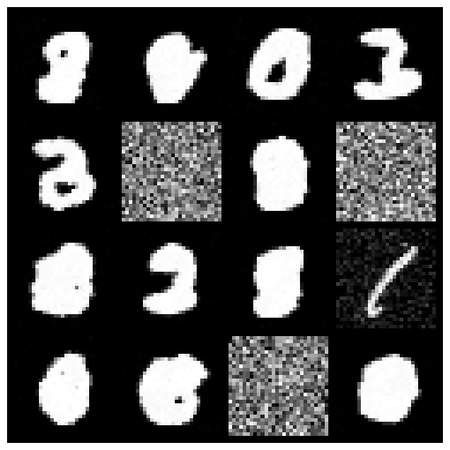1k5 images, U-netdim=32, no time, 500 epochs

The model learns the average of all digits, which gives this blurry shape (underfit), or sometimes it doesn’t find the right direction in the space and only generates noise.

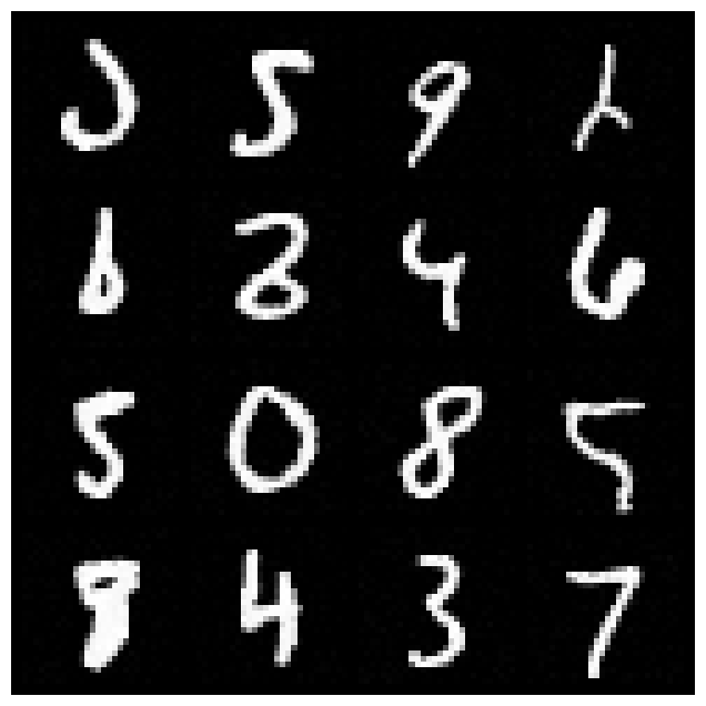same model, but with 700 epochs

We almost have real digits…

My second question was: “how does the model learn over time?”

This is where the interesting aspect of the DDPM paper’s “simple loss” comes in: If we keep the initial ELBO loss, small noises are a lot more weighted and larger t have are down-weighted, so the model trains more on small noises where the current distribution is already near the real one and not on the harder timestep where the model has to move in the right direction.
Using a uniform loss counterbalances this by equalizing learning across time.
An interesting measure would be the loss_t, the evolution of the loss for a signle timestep t across the training (You can find this loss in the related notebook: DDPM.ipynb.)

At first glance, these simple questions can seem pointless, but I find very interesting to remove part of a model to see how it reacts and how these parts change the model.

DDIM

From the previous experiments, we can see how sensitive the model is to the handling of timesteps and time, however a limitation of DDPM is the sampling where timesteps play the main role.
A main assumption of the model is that we have Gaussians as posteriors with small timesteps, so the more timesteps we use, the more this assumption holds.
For now, the model learns to denoise gradually, but that means when we sample, we need to do 300 passes with the model (I chose 300 timesteps) which takes time when you want to generate several images.

At a larger scale and on high-resolution images (not 28×28 like MNIST), the difference in sampling time is abyssal between DDPM and GAN: “For example, it takes around 20 hours to sample 50k images of size 32 × 32 from a DDPM, but less than a minute to do so from a GAN on an Nvidia 2080 Ti GPU.” Song et al.

Before moving to DDIM, I tried simply skipping steps in the classic DDPM sampling instead of going one by one, but it was very disappointing.

The main insight of DDIM is that the loss doesn’t depend on the joint distribution $\color{green}{\boldsymbol{q(x_1,\ldots,x_T \mid x_0)}}$, but only on the $\color{green}{\boldsymbol{q(x_t \mid x_0)}}$.
In the reverse process, we go one by one to follow the inverse Markov chain, because that’s what the joint distribution $q(x_1,\ldots,x_T \mid x_0) = q(x_T \mid x_0)\prod_t q(x_{t-1} \mid x_t,x_0)$ imposes on us, but the loss is actually much less constraining. This is where the Gaussian property “the nice property” is magical, we have a direct link between $x_t$ and $x_0$. Without these Gaussian factorizations, we would be forced to follow the inverse distribution $q(x_{t-1} \mid x_t)$.
The idea of DDIM is to see that we can choose a different process with a different joint distribution, but which has the same marginals $q(x_t \mid x_0)$, giving exactly the same loss. They thus use a deterministic sampling (non-Gaussian as in DDPM where noise is added at each timestep) and take $T/S$ steps instead of $T$.
This wasn’t conclusive in DDPM due to the added noise (stochasticity).
We still can’t jump from $T$ to $0$ directly though, our model breaks down information progressively even with DDIM.

What’s interesting to note, however, is that DDIM requires a better model to sample as well as DDPM. The noise added in DDPM during sampling can correct the model’s error, which slows down error accumulation throughout sampling.
The error will propagate in DDIM because it has become deterministic and we no longer have this stochasticity.

With enough data, I manage to divide the number of steps by 5 without too much quality loss:

Unet=64, 4k images, 700 epochs, S=5

The output is however less varied than classic DDPM, which is due to the deterministic nature of sampling and the fact that the model is still trained on few data:

same model but DDPM

Classifier-free guidance

We now know how to learn a distribution and sample, but we’re sampling a random image. We’d like to condition and choose what we sample.
For that, we do classifier guidance or here classifier-free guidance (you’ll see why in a few lines).
Geometrically, it’s fairly simple if we adopt the score view ($\nabla \log p_{t}(x_t)$): The score lets us navigate in the space towards the distribution. Our DDPM loss actually comes down to learning the score, or at least it’s equivalent (cf Score matching Y.Song). (This comes from Tweedie’s formula)

Using Bayes, we directly get:

\[\color{yellow}{ \nabla \log p(x_t \mid y) = \nabla \log p(x_t) + \nabla \log p(y \mid x_t)}.\]

And it’s the second term that corresponds to a classifier that lets us go towards a chosen place in the distribution.
Now, we won’t train an external classifier here but train the model half the time with the conditioning as data during training and the other half without conditioning.
The classifier is internal to the model, hence the name classifier-free guidance (cfg).
This way, we can add both contributions and navigate correctly in the space.

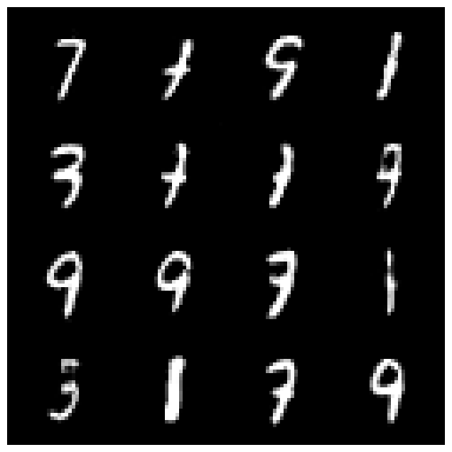
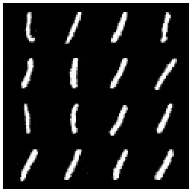Conditioning on 1 in the space

References

• Ho, J., Jain, A., & Abbeel, P. (2020). Denoising Diffusion Probabilistic Models. NeurIPS 2020. arxiv.org/abs/2006.11239
• Song, J., Meng, C., & Ermon, S. (2020). Denoising Diffusion Implicit Models. ICLR 2021. arxiv.org/abs/2010.02502
• Song, Y., & Ermon, S. (2019). Generative Modeling by Estimating Gradients of the Data Distribution. NeurIPS 2019. arxiv.org/abs/1907.05600
• Weng, L. (2021). What are Diffusion Models? Lilian Weng’s Blog. lilianweng.github.io/posts/2021-07-11-diffusion-models