Regression Ridge

Repo Github Ridge

Introduction

Let’s start from the beginning: OLS regression (Ordinary Least Squares), the standard linear regression and a classic in any statistics course. As a reminder, the closed-form estimator is $\hat{\beta} = (X^{\top} X)^{-1} X^{\top} y$

$X \in \mathbb{R}^{n \times p}$ is the matrix of explanatory variables (design matrix), $y \in \mathbb{R}^{n}$ is the observation vector, $\hat{\beta} \in \mathbb{R}^{p}$ is the estimator of the model parameters, $n$ is the number of observations, $p$ is the number of parameters (explanatory variables, intercept included).

Recall the assumptions:

\[y = X\beta + \varepsilon, \qquad \varepsilon \sim \mathcal{N}(0, \sigma^2 I_n).\]

What’s really useful for understanding the issues with OLS is the Singular Value Decomposition (SVD). Using it, we get directly that

\[\operatorname{Var}\!\left(\hat{\beta}_{\mathrm{OLS}}\right) = \sigma^{2} V \operatorname{diag}\!\left(\frac{1}{\lambda_1},\dots,\frac{1}{\lambda_i}\right) V^{\top}\]

where $\lambda_i = \gamma_{i}^2$ with $\gamma_i$ the singular values of $X$. Working in the eigenbasis, we focus on the coefficients $\frac{1}{\lambda_{i}}$. We can see that if any of them is zero, i.e. we have collinearity, the variance associated with that parameter diverges (in the corresponding eigendirection) and corrupts the model. On top of that, the estimated error variance depends on both n and p:

\[\hat{\sigma}^2 = \frac{1}{n - p} \left\lVert y - X\hat{\beta} \right\rVert^2\]

If $p>n$, $X^{\top} X$ is no longer invertible and the estimator is no longer unique. If $p=n$, we have no degrees of freedom left, $\hat{\sigma}^2$ becomes undefined and we can no longer estimate $\sigma$, the model becomes non-identifiable (and therefore meaningless). Finally, if $X^{\top}X$ is ill-conditioned, the model becomes unstable and unusable.

That’s why we turn to Ridge, which addresses both issues at once: reducing dimensionality while shrinking unnecessary parameters.

Ridge

Raw Model

Ridge isn’t free: we’ll certainly reduce the variance of our estimators, but we’ll also increase their bias.

The idea behind Ridge is to add an $L^2$ penalty controlled by a hyperparameter $\alpha \ge 0$ (called “shrinkage”: we constrain the range of values the estimated parameters can take) to our optimization problem:

\[\hat{\beta}_{\text{ridge}} = \arg\min_{\beta} \left( \| y - X\beta \|_2^2 + \alpha \| \beta \|_2^2 \right)\]

This makes the problem well-posed regardless of the values of $p$ or $n$, or whether we have collinear variables. We force good conditioning, $X^{\top}X + \alpha I$ is invertible, and we bound the variance.

Understanding the Model

Bayesian Approach

First, let’s ask ourselves why we add a term $\alpha |\beta|_2^2$. This can be understood through the Bayesian approach to statistics, Ridge actually turns out to be equivalent to MAP (Maximum A Posteriori) estimation:

We start with Bayes’ theorem and take the log: $\log P(\theta \mid X, y) = \log P(X, y \mid \theta) + \log P(\theta) - \log P(X, y)$ where $X, y$ are the observations and $\theta$ is the parameter.

Here, we want to maximize $\log P(\theta \mid X, y)$ or equivalently minimize the cost $J(\theta) = -\log P(\theta \mid X, y)$, so we maximize $\log P(X, y \mid \theta) + \log P(\theta)$.

We recover our two cost function terms: $-\log P(\theta)$ for regularization and $-\log P(X, y \mid \theta)$ for the OLS term.

Going further, one can show that $P(X, y \mid \theta) = \mathcal{N}(y \mid X\theta, \sigma_1^2), \quad P(\theta) = \mathcal{N}(\theta \mid 0, \sigma_2^2)$ corresponds exactly to the cost function defined in the previous section.

What’s fundamental and really interesting here is that by doing Ridge, we’re assuming $\theta$, or in our case $\beta \sim \mathcal{N}(0, \tau^2 I)$.

We’re therefore assuming that our model corresponds to many small effects adding up together, Ridge = Gaussian prior. From this, the properties and quirks of Ridge become clear (for example, the penalty only depends on the norm, not the direction, because a Gaussian is rotation-invariant!).

End of the statistics interlude.

Cost Approach

To properly see all the advantages of Ridge, we go back to the singular values of $X$.

The unique solution to the problem is: $\hat{\beta} = (X^{\top} X+\alpha I)^{-1} X^{\top}y$ This time the estimator is biased:

\[\mathbb{E}[\hat{\beta}] = (X^{\top} X+\alpha I)^{-1} X^{\top} X\, \beta\]

and working in the eigenbasis, $\mathbb{E}[\hat{\beta_i}] = \frac{\gamma_{i}^2}{\gamma_{i}^2 + \alpha} \beta_i$, giving a bias $\operatorname{Bias}(\hat{\beta}_i)= -\frac{\alpha}{\gamma_i^2 + \alpha}\,\beta_i$ (*)

We can see that the bias is nonzero as long as $\alpha > 0$, and moreover it is bounded (in absolute value) by “the true coefficient”, with the bound reached when $\alpha \to +\infty$. This makes sense: if $\alpha = \infty$, we crush all estimated coefficients down to zero.

Similarly for the variance:

\[\operatorname{Var}(\hat{\beta}) = \sigma^2 (X^\top X + \alpha I)^{-1} X^\top X (X^\top X + \alpha I)^{-1}\]

and switching to SVD:

\[\operatorname{Var}(\hat{\beta}_i) = \sigma^2 \frac{\gamma_i^2}{(\gamma_i^2+\alpha)^2}\]

We can clearly see that the variance has decreased compared to the OLS model, and that it decreases as $\alpha$ grows. Moreover, when $\gamma_i = 0$, both the variance and the expectation are zero, the coefficient is then zero with probability 1.

In practice, a few precautions are needed with Ridge:

• We normalize the $x_i$ so they become centered and scaled, ensuring the penalty is applied fairly and avoiding high-variance observations having too much influence (without normalization, they would be much less penalized since $\gamma_i$ would be large and the shrinkage factor (*) would be close to 1).
• We then center the target variable y so the intercept isn’t penalized. Since the $x_i$ are centered, the intercept equals the mean of y and can simply be removed. No penalty will therefore be applied to the intercept, indeed, it doesn’t represent an association between the target variable and an explanatory variable.

Model Implementation

Time for the from-scratch implementation.

def __init__(self,X):

        self.X       =  X
        self.mu_X    =  self.X.mean(axis=0)
        self.sigma_X =  self.X.std(axis=0, ddof=0)
        self.Xc      =  (self.X - self.mu_X) / self.sigma_X

        self.U, self.d, self.Vt = np.linalg.svd(self.Xc, full_matrices=False)
        
        self.V       =  self.Vt.T
        self.Xct     =  self.Xc.T

The model is defined from the observations X, and we’ll use the target y in fit.

First we normalize X as discussed earlier. This step could have gone inside fit, but since I mainly wanted a function that tests several values of $\alpha$ (see below), I kept it in init to save redundant computation.

Then, to avoid recomputing the inverse of a matrix that depends on $\alpha$ non-explicitly, we use the SVD which gives us a closed-form formula knowing V and U. The full_matrices=False parameter computes the economy SVD (keeping only nonzero singular values), avoiding unnecessary dimensions when n != p without losing any relevant directions.

The second important method is fit:

def fit(self, y,alpha):

        self.mu_y = y.mean()
        yc = y - self.mu_y
        shrink = self.d / (self.d**2 + alpha)
        beta_s = self.Vt.T @ (shrink * (self.U.T @ yc))
        self.coef = beta_s / self.sigma_X
        self.intercept = self.mu_y - self.mu_X @ self.coef
        return self.coef, self.intercept

We first center y, then compute the estimate for our standardized model using our SVD-simplified closed-form formula. We then come back to our actual model, standardization being bijective with nonzero standard deviation:

\[y_s = X_s \beta_s, y_s = y-\mu_y, X_s = \frac{X-\mu_X}{\sigma_X}, y = \frac{X}{\sigma_X} \beta_s + \mu_y - \mu_{X}^{\top}\beta_s\]

Note that we handled the intercept separately so it doesn’t get penalized. We can now make predictions. (the predict function is on GitHub, along with all the code presented and needed for this post)

Prediction

Here we’ll compare OLS and Ridge on data represented by 2 points that we’ll add noise to, in order to show that Ridge is much more robust and produces more stable coefficients (since the variance is reduced).

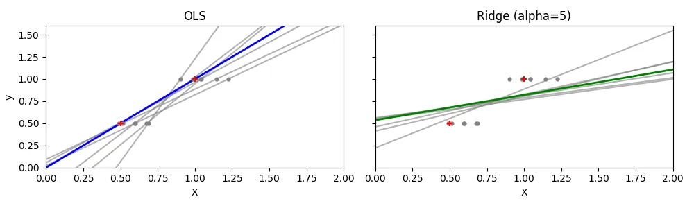
We created 6 noisy realizations and 1 noise-free realization of the dataset, fitting one model (OLS and Ridge) per realization. This is what we see in the plots above: the Ridge predicted lines are much closer to each other. Here OLS completely overfits (the model learns the noise), exactly what Ridge prevents. We do lose something in bias, but we gain in generalization. The green and blue curves correspond to the noise-free observation.

Scikit-learn doesn’t directly handle data standardization (you need to use StandardScaler() separately), but our from-scratch model does it as soon as a model is initialized (ridge(X)). We could have put the standardization inside fit, but since we have a function testing a range of alpha values, this avoids redoing the standardization at every fit call.

X_train = np.array([[0.5], [1.0]])
y_train = np.array([0.5, 1.0])

alpha = 5
X_plot = np.array([[0],[2]])
noises = 0.1 * np.random.normal(size=(6,) + X_train.shape)
for eps in noises:
    this_X = X_train + eps
    rd = ridge(this_X)
    rd.fit(y_train, alpha)

The question now is how to choose $\alpha$. In the comparison above I picked $\alpha$ by eye, but $\alpha$ is a hyperparameter and we want the optimal one. Optimal with respect to what? With respect to prediction error, so the residuals, RSS, RSSE, or any other metric quantifying error. Two approaches work here: test the model on a test set and find the $\alpha$ that minimizes error on it, or use cross-validation (when data is scarce).

Here we’ll test on the california_housing dataset, where OLS actually works reasonably well despite some correlated features. We split the dataset in two:

X_train, X_test, y_train, y_test = train_test_split(
    X, y, test_size=0.25, random_state=42)

We first find the optimal alpha using the find method in the ridge class:

    def rss(self, X_t, y_t):
        y_pred = X_t @ self.coef + self.intercept
        return np.sum((y_t - y_pred)**2)
    def find(self, mx, n, X_val, y_val, y_train):
        
        J=np.logspace(-4, np.log10(mx), n)

        rssm=np.inf
        self.rm=[]
        self.v=[]
        self.best_alpha=None

        for alpha in J:
            self.fit(y_train, alpha)
            b=self.rss(X_val, y_val)
            self.rm.append(b)
            self.v.append(alpha)
            if b<rssm:
                rssm=b
                self.best_alpha=alpha

        return self.best_alpha,rssm

We provide a maximum value $\alpha_{max}$ and find trains a model for each $\alpha$ in J, where J is a logarithmic discretization of the interval $[10e-4, \alpha_{max}]$. We then look for the $\alpha$ that minimizes RSS and compare against OLS RSS.

Results:

• Best alpha : 168.3
• RSS Ridge : 2780.0
• RSS OLS : 2792.2

We do observe an improvement thanks to Ridge (for better stability of the RSS and results, cross-validation would have been more appropriate). Finally we plot the RSS as a function of alpha.

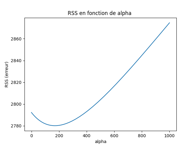
We can clearly see that there’s a sweet spot between an unstable OLS and overly aggressive generalization. That’s exactly what the hyperparameter $\alpha$ controls.